A Simple Example¶

The simplest scenario involves providing a sequence and a secondary structure as input and obtaining coarse-grain tertiary structures as output. The input will be a fasta file augmented with secondary structure, which we will store as 2mis.fa:

>2mis
GAGCUGCAGCACGAAAGUGACGGCUC
((((((...(((....))).))))))

With this, we can invoke ernwin using the ernwin.py script:

ernwin.py 2mis.fa --iter 1000

This will start the sampling engine. On the commandline you will see a warning that sampling is starting from scratch (because the fasta file does not contain an initial structure to start from), followed by one line printed for each sampling step. The simulation should not take more than 5 minutes. It creates an output directory with the id of the provided sequence (taken from the fist line of the fasta file, 2mis, in this case). This directory contains an initial 3D structure created by ernwin (build000001.coord), the commandline arguments used inside version.txt and a subdirectory simulation01. This directory then contains the top 3 lowest energy sampled structures (best0.coord until best3.coord) and one structure saved every 100 steps. The format for these structures is described in the documentation of the forgi package. They can be visualized using the visualize_cg.py script provided by forgi (which depends on PyMOL):

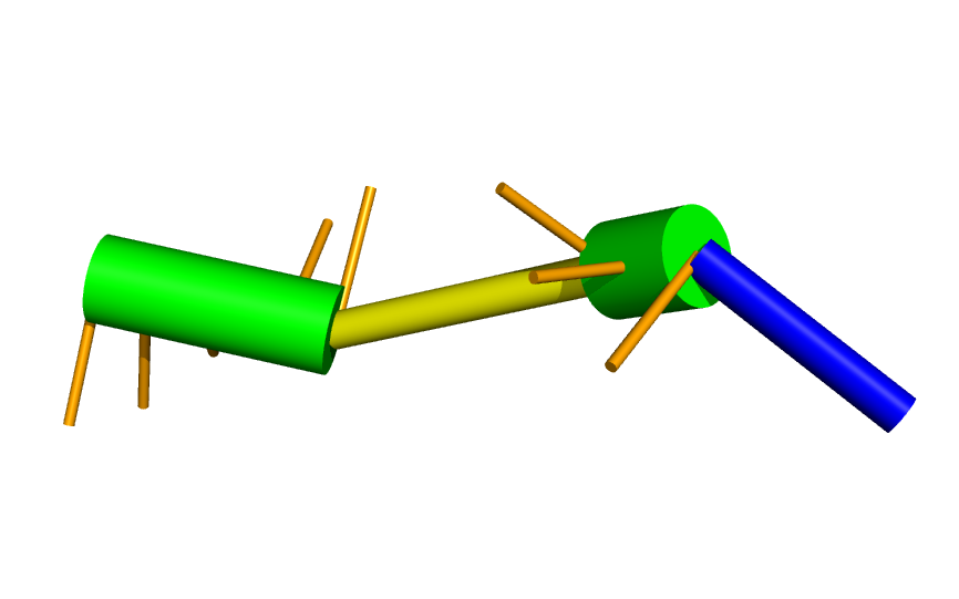
visualize_rna.py 2mis/simulation_01/best0.coord

To yield something like this:

We can also compare it to the native structure (in dark green):

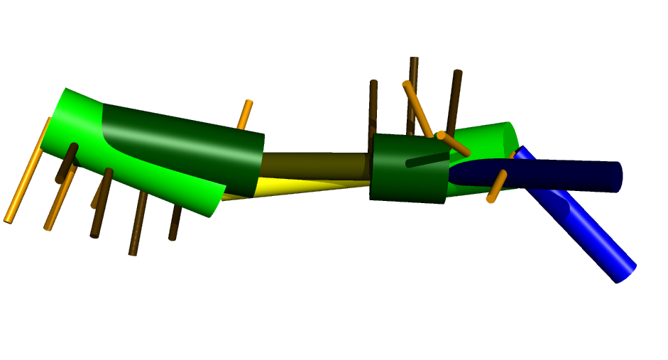
This was generated by first extracting the coarse grain representation from the pdb file (using forgi), then visualizing and aligning (using the --align option of visualize_rna.py):

rnaConvert.py -T forgi 2mis.pdb > 2mis_native.cg
visualize_rna.py 2mis/simulation_01/best0.coord 2mis_native.cg --align

Sampling from an Existing CG File¶

For benchmarking purposes, it’s often easier to start with the native structure. This allows one to monitor the RMSD between the current sampled structure and the native as the simulation progresses. Doing so is almost identical to starting from a fasta file, wherein the argument to ernwin.py is the cg file instead:

ernwin.py 2mis_native.cg --iter 1000

To create a cg file from a pdb file, see the example in the previous section or the relevant documentation for the forgi package.

Sampling with all-atom reconstruction¶

Often, you will need all-atom PDB files tu further analyze the results or put them into other tools for further refinement/ evaluation.

To run the above simulation with all-atom reconstruction every 100 steps, use the following command:

ernwin.py 2mis.fa --iter 1000 --reconstruct-every-n 100 --reconstruction-pdb-dir ernwin_data/PDBs --reconstruction-cg-dir ernwin_data/CGs

and optionally (for speed-up) add --reconstruction-cache-dir ~/.cache/ernwin

The two directories you have to give have to contain the correct files, as described in the previous section.

In addition to the coord files, this will also create 10 pdb files along the sampling trajectory. As these PDB files are created by sticking fragments together, they can contain clashes or gaps between residues. SPQR can be used to mend these gaps, as described in [1].

The Log File¶

As ernwin runs, it outputs diagnostic information about the sampling procedure. The same information can be found in the output folder in the out.log file

References

[1] Thiel, B.C., Bussi, G., Poblete S and Hofacker, I.L. Sampling globally and locally correct RNA 3D structures using ERNWIN, SPQR and experimental SAXS data bioRxiv 2022.07.02.498583; doi: https://doi.org/10.1101/2022.07.02.498583