- Usage Reference
Application Usage Examples
This chapter gives some short instructions to use the command-line program and two example applications. The SBML file that is used as an example (MAPK.xml) is a slightly modified version taken from the SBML model repository after a model by Boris Kholodenko, 2000 (PubMed abstract). Please see the information in the following paragraphs to find the applications that are described here on your system.
Please see the full reference guide for these applications below to learn about all options and possibilities of the applications.
Windows Binaries and Visual C++ Project
The applications described below are contained in the release.zip file (and should be extracted) or if you have built the source from SBML_odeSolver-x.x.tar.gz using the CompleteSOSLib.sln using the release configuration then the applications will reside in <SBML_odeSolver>\Win32\release. To be able to run these applications as described below follow the directions here so that the path variable includes either <SBML_odeSolver>\Win32\release or the directory in which the contents of the zip file reside. The MAPK.xml model is contained in either of those directories.
Installation from Source Code (Unix, MinGW)
If you build SOSlib from source code you will find the application odeSolver in the folder `odeSolver' and wherever you installed it to (with `configure --prefix=PATH and `make install'). The applications Sense and ParameterScanner and the SBML file MAPK.xml are in the `examples' folder. The script gnuplotscript.awk can be found in the `scripts' folder.
Background Information
If you are unfamiliar with or want to learn more about either the
command-line in general, the plotting tool gnuplot or the scripting
language awk please follow the links to external tutorials below.
If you are a Windows user and don't even know
where to find your command-line, please see our Short Command-line Tutorial for Windows
Users.
odeSolver / SBML_odeSolverApp
The command-line application odeSolver (if you installed the Windows
binaries or built from the Visual C++ project it is called
SBML_odeSolverApp.exe) is the main application of the SOSlib, implementing
most functionalities of the SOSlib library.
Please run the odeSolver
with option -h or --help to learn about rich input options, or see the full
reference below.
Simulating an SBML Model
To simulate a model type a command similar to the following in the shell:
| Linux: | odeSolver MAPK.xml --time 1500 --printstep 200 > MAPK.txt |
| Windows: | SBML_odeSolverApp MAPK.xml --time 1500 --printstep 200 > MAPK.txt |
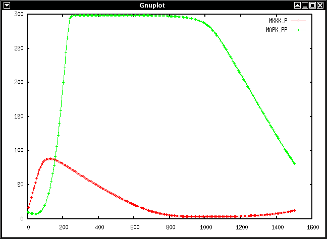
To display the results we need to first create a gnuplot file from the model output using the following command:
gnuplotscript.awk MAPK.txt MKKK_P MAPK_PP > MAPK.gnuplot
This generates a gnuplot script to display the data in MAPK.txt for the
time course of MKKK_P and MAPK_PP
To display the plot type the command:
| Linux: | gnuplot -persist MAPK.gnuplot & |
| Windows: | wgnuplot -persist MAPK.gnuplot & |
This procedure should make gnuplot open the following figure in a new window:
Result Visualization with XMGrace Module
NOTE: Currently, no one has ever installed SOSlib with the XMGrace module on Windows. Please report us if you have managed to do this! The version of SBML_odeSolverApp included in the release.zip file does not include the Grace module. The Visual C++ project and solution files do not build applications which include the Grace library.
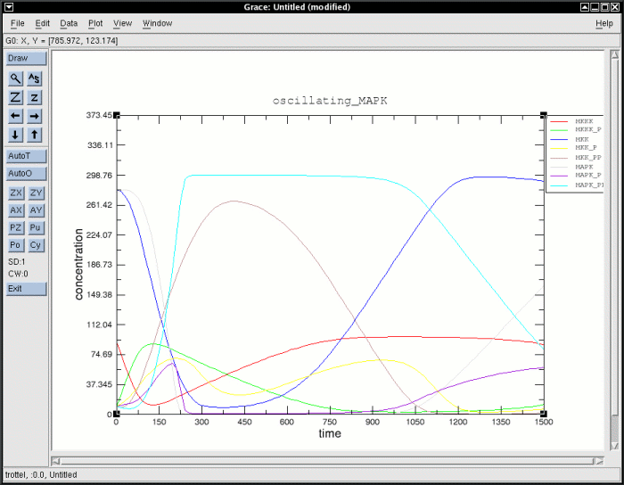
If you have installed SOSlib with the optional XMGrace module, you can directly sent integration results to XMGrace with the option -x. The command
odeSolver MAPK.xml --time 1500 --printstep 100 -x
will open a new XMGrace window as shown in the following figure:
Output of the optional XMGrace module
Graph Drawing with GraphViz Module
NOTE: Currently, no one has ever installed SOSlib with the Graphviz module on Windows. Please report us if you have managed to do this! The version of SBML_odeSolverApp included in the release.zip file does not include the Graphviz module. The Visual C++ project and solution files do not build applications which include the Graphviz library.
If you have installed SOSlib with the optional graph drawing module based
on Graphviz
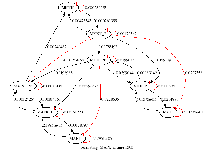
you can draw not only
the usual bipartite reaction network graph (with option -g) in various
formats, but also a species interaction graph based on the
non-zero entries of the Jacobian matrix of the ODE system J =
δf(x)/δx(with option -m) at the endtime of a specific
simulation run. Such graphs can at least for small models be very
informative about possible negative and positive feedback loops which
usually define a reaction networks dynamics. In the figure below you can
e.g. find the negative feedback that is responsible for the oscillatory
behaviour of this model.
A parameter dependance graph can currently
not be drawn via the command-line application, but an example application
(analyzeSensitivity), which draws such a graph is
available in the `examples' folder.
The command
odeSolver MAPK.xml --time 1500 --printstep 1 -m --gvformat gif
will save the following figure as `MAPK.xml_jm.gif':
Species interaction graph generated by the optional Graphviz graph layout module
Interactive Mode
The option -i will allow you to enter the interactive mode of the odeSolver command-line applications. If you press `h' you will get a list of all functions you can call from this mode. This mode is sometimes helpful if you want to quickly explore a new model. You can view initial conditions, reactions and rules, the constructed ODE system, the Jacobian matrix, and you can of course integrate the model as often as you want, and display results in XMGrace or draw graphs. You can also set new initial conditions to all species.
ParameterScanner
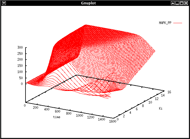
To generate a 3D plot of a species concentration over time series for a range of parameter or species concentrations type a command as follows:
ParameterScanner MAPK.xml 200 7.5 Ki 0 15 0.15 MAPK_PP > pscan.gnuplot
This creates plot data of a parameter scan in MAPK.xml of parameter Ki
from 0 through 15 in steps of 0.15.
The surface plotted is the concentration of MAPK_PP in 200 timesteps of 7.5
time units.
To display the plot type the command:
| Linux: | gnuplot -persist pscan.gnuplot & |
| Windows: | wgnuplot -persist pscan.gnuplot & |
This procedure should make gnuplot open the following figure in a new window:
Sensitivity
To perform solution forward sensitivity analysis type a command as follows:
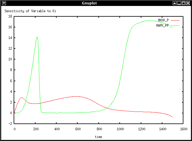
Sense MAPK.xml 200 7.5 p Ki MKKK_P MAPK_PP > sense.gnuplot
This creates a plot of the sensitivity of species MKKK_P and MAPK_PP to the
values of the parameter Ki for the timecourse of 200 timesteps of 7.5 time
units.
To display the plot type the command:
| Linux: | gnuplot -persist sense.gnuplot & |
| Windows: | wgnuplot -persist sense.gnuplot & |
This procedure should make gnuplot open the following figure in a new window:
Alternative one can type a command as follows:
Sense MAPK.xml 200 0.5 v MAPK_PP Ki V1 K1 > sense.gnuplot
This creates a plot of the sensitivity of species MAPK_PP to the values of the parameters Ki, V1 and K1 for the timecourse of 200 timesteps of 0.5 time units.
See the full reference for this application below for an important crash warning.
Learning more about 3rd Party Tools
You can learn more about the various 3rd party tools used above at the following external websites:
The Bash Shell
Quick Guide to Writing Bash ScriptsComprehensive Guide to Writing Bash Scripts
GNUPLOT
Gnuplot IntroductionGnuplot FAQ
Gnuplot Not So FAQ (a great and comprehensive tutorial)
AWK
Awk ReferenceAwk User Guide
Reference Guide to SOSlib Applications
odeSolver / SBML_odeSolverApp
This executable can be excuted with a command of the following form:
| Linux: | odeSolver <SBML File> [OPTIONS] |
| Windows: | SBML_odeSolverApp <SBML File> [OPTIONS] |
where all possible options can be printed out with option -h or --help as follows
| GENERAL OPTIONS | ||
| -h | --help | Print (this) usage information. |
| -i | --interactive | Turn on interactive mode |
| --gvformat <Str> | Set output format for graph drawings (now set to: ps); ignored if compiled w/o graphviz) | |
| SBML FILE PARSING | ||
| -v | --validate | Validate SBML file before further processing |
| --model <Str> | SBML file name (not needed! see USAGE) (now set to: ) | |
| --mpath <Dir> | Set Model File Path (now-set to: ./) | |
| --schema11 <Str> | Set filename for SBML schema Level 1 Version 1 (now set to: sbml-l1v1.xsd) | |
| --schema12 <Str> | Set filename for SBML schema Level 1 Version 2 (now set to: sbml-l1v2.xsd) | |
| --schema21 <Str> | Set filename for SBML schema Level 2 Version 1 (now set to: sbml-l2v1.xsd) | |
| --spath <Dir> | Set schema file path, absolute or relative to model path (now set to: ./) | |
| (1) PRINT REACTIONS AND DERIVED ODEs | ||
| -e | --equations | Print Reactions and derived ODE system |
| -o | --printsbml | Construct ODEs and print as SBML model |
| -g | --modelgraph | Draw bipartite graph of reaction network (to .dot text file if compiled w/o graphviz) |
| (2) INTEGRATING | ||
| -f | --onthefly | Print results during integration |
| -l | --message | Print messages, and integration statistics |
| -j | --jacobian | Toggle use of the jacobian matrix or CVODE's internal approximation (default: jacobian) |
| -s | --steadyState | Abort integration at steady states |
| -t | --sensitivity | activate sensitivity analysis (default: no) |
| -n | --event | Do not abort on event detection, but keep integrating. ACCURACY DEPENDS ON --printstep!! |
| --printstep <Int> | Time steps of output, or (now set to: 50) | |
| --time <Float> | Integration end time (now set to: 1) | |
| --error <Float> | Absolute error tolerance during integration (now set to: 1e-009) | |
| --rerror <Float> | Relative error tolerance during integration (now set to: 0.0001) | |
| --mxstep <Int> | Maximum step number during integration (now set to: 10000) | |
| (3) INTEGRATION RESULTS | ||
| -a | --all | Print all available results (y/k/r + conc.). |
| -y | --jacobianTime | Print time course of jacobian matrix entries, instead of concentrations |
| -k | --reactions | Print time course of the reactions (kinetic laws) instead of concentrations |
| -r | --rates | Print time course of the ODEs, instead of concentrations |
| -w | --write | Write results to file (path/modelfile.xml.dat) |
| -x | --xmgrace | Print results to XMGrace; uses SBML Names instead of Ids (ignored if compiled w/o Grace) |
| -m | --matrixgraph | Draw species interactions from the jacobian matrix at last timepoint of integration (to .dot text file if compiled w/o graphviz) |
ParameterScanner
This command generates a gnuplot surface plot which contains the effect of a range of values of a given parameter on the simulated time series of a given species.
The command line for this executable has the following form:
ParameterScanner sbml-model-file time-steps time-step-length parameter parameter-start parameter-end parameter-step species [absolute-error-tolerance] [relative-error-tolerance] [maximum integration steps]
where 'time-steps' is the number of time steps to take
where 'time-step-length' is the interval in simulation time between time
steps
where 'parameter-start' is the lower bound on the scanned range of
parameter values
where 'parameter-end' is the upper bound on the scanned range of
parameters values
where 'parameter-step' is the interval between sampled parameter values
where 'species' is the species whose concentration is plotted as a
surface
The gnuplot output is simply printed to the standard output stream.
Sensitivity (Sense)
This command generates a gnuplot 2D file which plots the forward solution sensitivity of one or more species concentrations to one or more parameters. The command line for this executable has the following form:
Sense sbml-model-file time-steps time-step-length mode symbol [symbols] [absolute-error-tolerance] [relative-error-tolerance] [maximum integration steps]
where 'time-steps' is the number of time steps to take
where 'time-step-length' is the interval in simulation time between time
steps
mode is either 'p' or 'v'.
If mode is 'p' then the sensitivies of one
or more
given species to a given parameter is displayed.
If mode is 'v' then
the sensitivies
of a given species to one or more given parameters is displayed.
symbol is a variable (non constant species, compartment or parameter) if
mode is 'v'.
symbol is a parameter if mode is 'p'
symbols is a sequence of parameters if mode is 'v'
symbols is a sequence of variables if mode is 'p'
The gnuplot output is simply printed to the standard output stream.
WARNING: Sense will crash, if you choose a variable instead of parameter for sensitivity analysis.
Scripts
This command generates a gnuplot plot file on standard output from the default output of SBML_odeSolverApp. This command has the form:
gnuplotscript.awk output-file species
where `output-file' contains the output of odeSolver/SBML_odeSolverApp
and
`species' is a sequence of species ids which are required for
plotting.
The generated gnuplot script simply refers to the content of the output-file so don't delete the output-file if you want to plot the results in the future.
